Supervised learning in a single-layer neural network
Let's consider a
single-layer neural network with b inputs and c outputs:
- Wij = weight from input i to unit j in output layer;
Wj is the vector of all the weights of the j-th neuron in
the output layer.
- Ip = input vector (pattern p) =
(I1p, I2p, ...,
Ibp).
- Tp = target output vector (pattern p) =
(T1p, T2p, ...,
Tcp).
- Ap = Actual output vector (pattern p) =
(A1p, A2p, ...,
Acp).
- g() = sigmoid activation function: g(a ) = [1 + exp
(-a)]-1
Supervised learning
We have seen that
different weights of a neural network produce different functions of the input.
To train a network, we can present some sample inputs and compare the actual
output to the desired results. The difference is called the error.
![[an error term is computed and fed back]](Perceptron.files/learning.gif) The different
learning rules tell us which way to adjust the weights to reduce this
error. We say that training has converged when this error reaches some
small, acceptable level.
The different
learning rules tell us which way to adjust the weights to reduce this
error. We say that training has converged when this error reaches some
small, acceptable level.
Often the learning rule takes the following form:
Wij (t+1) = Wij (t) +
eta . err (p)
where 0 <= eta < 1 is a parameter that
controls the learning rate, and err(p) is the error when input pattern
p is presented.
[Back to
the Adaline/Perceptron/Backprop applet page]
Adaline learning
ADALINE is an acronym for ADAptive
LINear Element (or ADAptive LInear NEuron). It was developed by Bernard
Widrow and Marcian Hoff (1960).
The adaline learning rule (also known as the least-mean-squares rule, the
delta rule, and the Widrow-Hoff rule) is a training rule that minimises the
output error using (approximate) gradient descent. After each training pattern
Ip is presented, the correction to apply to the weights
is proportional to the error. The correction is calculated before
the thresholding step, using errij
(p)=Tp-Wij Ip:
Thus, the weights are adjusted by
Wij (t+1) = Wij (t) +
eta (Tp-Wij Ip)
(Ip)
This corresponds to gradient descent on the quadratic
error surface, Ej=Sump [Tp
- Wj . Ip] 2
[Back to
the Adaline/Perceptron/Backprop applet page]
Perceptron learning
In perceptron learning, the
weights are adjusted only when a pattern is
misclassified. The correction to the weights after
applying the training pattern p is
Wij (t+1) = Wij (t) + eta (Tp
- Ap) (Ip)
This corresponds to
gradient descent on the error surface E (Wij )=
Summisclassified [Wij
(Ap)(Ip)].
[Back to
the Adaline/Perceptron/Backprop applet page]
Pocket algorithm
The perceptron learning algorithm
does not terminate if the learning set is not linearly separable. In many
real-world cases, however, we want to find the "best" linear separation
even when the learning sets are not ideal. The pocket algorithm is a
modification of the perceptron rule proposed by S. I. Gallant (1990). It stores
the best weight vector so far in a "pocket" while continuing to learn. The
weights are actually modified only if a better weight vector is found.
[Back to
the Adaline/Perceptron/Backprop applet page]
Backpropagation
The backpropagation
algorithm was developed for training multilayer perceptron networks. In this
applet, we will study how it works for a single-layer network. It was
popularized by Rumelhart, Hinton and Williams (1986), although similar ideas had
been developed previously by others (Werbos, 1974; Parker, 1985). The idea
is to train a network by propagating the output errors backward through the
layers. The errors serve to evaluate the derivatives of the error function with
respect to the weights, which can then be adjusted.
The backpropagation algorithm for a single-layer network using the
sum-of-squares error function consists of two phases:
- Feedforward - apply an input; evaluate the activations
aj and store the error deltaj at each node
j
aj = Sum
i(Wij (t)
Ipi)
Apj = g (aj )
deltaj =
Apj -Ipj
- Backpropagation - compute the adjustments and update the
weights. Since there is just one layer, the output layer, we compute
Wij (t+1) =
Wij (t) - eta deltai
Ipj
(This is called "on-line" learning, because
the weights are adjusted each time a new input is presented. In "batch"
learning, the weights are adjusted after summing over all the patterns in the
training set.)
[Back to
the Adaline/Perceptron/Backprop applet page]
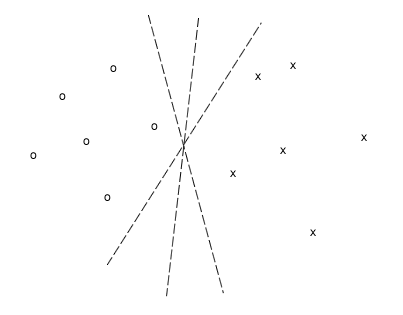
Optimal Perceptron learning
In the case of linear
separable problems a perceptron can find different solutions:
It would now be interesting
to find the hyperplane that assures the maximal safety tolerance:
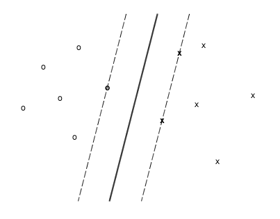
The margins of that hyperplane
touches a limited number of special points which define the hyperplane and which
are called the Support
Vectors.

The perceptron has to determine the samples for
which  . The remaining samples
with
. The remaining samples
with  are the Support Vectors sv.
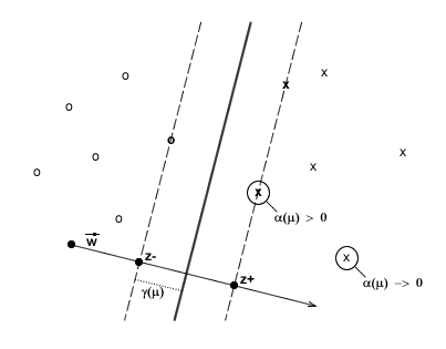
 Represents the distance between a sample and
 . z- and z+ represent the
projection of the critical points on the axis defined by
. z- and z+ represent the
projection of the critical points on the axis defined by .
.
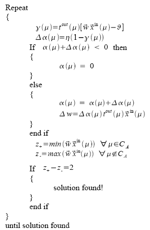
Algorithm of the Optimal Perceptron:
[Back to
the Adaline/Perceptron/Backprop applet page]
Further reading
- C. M. Bishop. Neural Networks for Pattern Recognition. Clarendon
Press, Oxford, 1995. pp 95-103 (adaline and perceptron); pp 140-148 (backprop)
- J. Hertz, A. Krogh, and R.G. Palmer. Introduction to the Theory
of Neural Computation. Addison-Wesley, Redwood City CA, 1991. pp 89-111
- R. Rojas. Neural Networks: A Systematic Introduction.
Springer-Verlag, Berlin 1996. pp 84-91 (perceptron learning); pp 159-162
(backprop)
[Back to
the Adaline/Perceptron/Backprop applet page]