Next | Top | JOS Index
| JOS Pubs |
JOS Home | Search
- Let
 be distributed according to a parametric family:
  . The goal is, given iid observations
  , to estimate
  . For instance, let be a series of coin flips where
  denotes ``heads'' and
  denotes ``tails''. The coin is weighted, so
  can be other than
  . Let us define
  ; our goal is to estimate . This simple distribution is given the name ``Bernoulli''.
- Without prior information, we use the maximum likelihood approach.
Let the observations be
 . Let
. Let  be the number of heads observed and
  be the number of tails.
- Not surprisingly, the probability of heads is estimated as the empirical
frequency of heads in the data sample.
- Suppose we remember that yesterday, using the same coin, we recorded 10
heads and 20 tails. This is one way to indicate ``prior information'' about
. We simply include these past trials in our estimate:
- As (H+T) goes to infinity, the effect of the past trials will wash out.
- Suppose, due to computer crash, we had lost the details of the experiment,
and our memory has also failed (due to lack of sleep), that we forget even the
number of heads and tails (which are the sufficient statistics for the
Bernoulli distribution). However, we believe the probability of heads is about
 , but this probability itself is somewhat uncertain, since we only
performed 30 trials.
, but this probability itself is somewhat uncertain, since we only
performed 30 trials.
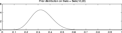
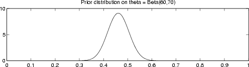
- In short, we claim to have a
 over the probability , which represents our prior belief. Suppose this distribution is
 and
and  :
:
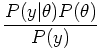
- Now we observe a new sequence of tosses:
 . We may calculate the posterior distribution
  according to Bayes' Rule:
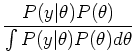
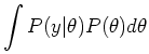
The term  is, as before, the likelihood function
of . The marginal
is, as before, the likelihood function
of . The marginal  comes by integrating out :
- To continue our example, suppose we observe in the new data
 a sequence of 50 heads and 50 tails. The
likelihood becomes:
a sequence of 50 heads and 50 tails. The
likelihood becomes:
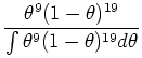
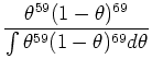
- Plugging this likelihood and the prior into the Bayes Rule expression, and
doing he math, obtains the posterior distribution as a
 :
:
- Note that the posterior and prior distribution have the same form. We call
such a distribution a conjugate prior. The Beta distribution is
conjugate to the binomial distribution which gives the likelihood of iid
Bernoulli trials. As we will see, a conjugate prior perfectly captures the
results of past experiments. Or, it allows us to express prior belief in terms
of ``invented'' data. More importantly, conjugacy allows for efficient
sequential updating of the posterior distribution, where the posterior
at one stage is used as prior for the next.
- Key Point The ``output'' of the Bayesian analysis is not a
single estimate of , but rather the entire posterior distribution. The posterior
distribution summarizes all our ``information'' about . As we get more data, if the samples are truly iid, the
posterior distribution will become more sharply peaked about a single value.
- Of course, we can use this distribution to make inference about
. Suppose an ``oracle'' was to tell us the true value of used to generate the samples. We want to guess
that minimizes the mean squared error between our guess and the true
value. This is the same criterion as in maximum likelihood estimation. We
would choose the mean of the posterior distribution, because we know
conditional mean minimizes mean square error.
- Let our prior be
 and
and
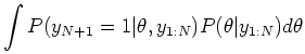
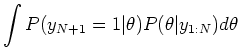
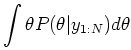
- The same way, we can do prediction. What is
 ?
?
Next | Top | JOS Index
| JOS Pubs |
JOS Home | Search
Download bayes.pdf
Download
bayes_2up.pdf
 [Automatic-links
disclaimer]
[Automatic-links
disclaimer]