Combination of drifts - "INTAS-OPEN-97-0606"

Reference Number: INTAS-97-0606

Development of an Intelligent Sensing Instrumentation Structure I.S.I.S.

Using Neural Networks in ISIS

Combination of drifts

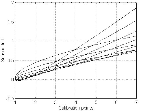
The third set of curves simulating a combination of two previous kinds of drifts is presented on Figure 7. The drift velocity of one part of sensors is increased and the velocity of other part of sensors is reduced in this case. Such kind of drift is not characteristic for the existing sensors, however it is expedient to research the method's possibilities for such data. As have researches shown, the model of single-layer perceptron does not provide acceptable results in this case. It is necessary to use non-linear neural networks for such drift data integration. The model of three-layer perceptron was used for experiment execution. The first layer of neural network contains 9 neurones, the second layer contains 9 neurones (with logistic activation function) and the third level contains one linear neurone. The training of multi-layer perceptron with data from Figure 7 is instability process and has shown different prediction results in calibration points. Therefore sum-squared error 10Å-4 and maximum training epoch number 30000 limited training per each neural network. It is necessary to note that the best convergence was shown by layer-by-layer training algorithm. 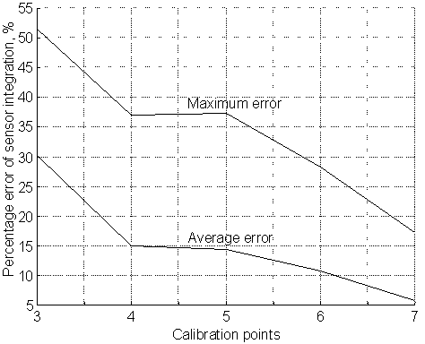The average training duration did not exceed 100 seconds per each curve. The maximum and average percentage errors of data integration (see Figure 8) did not exceed 52% and 30% accordingly.

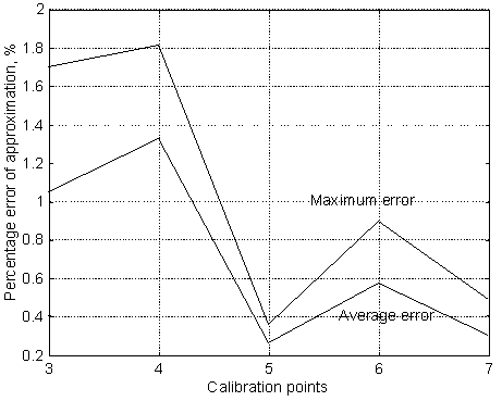
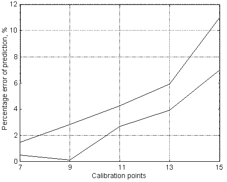
Figure 7. Third set of hypothetical data about sensor drift

Figure 8. Percentage integration error of third set of sensor drift

The results of historical data integration are approximated by special approximating neural network for correction factor prediction on sensor drift. Experimental researches (by simulation modelling) with using integration results considered above (only for drift "with saturation" from Figure 3) have shown that the percentage error of approximation is much lower than integration error. For example, approximating neural network (model of three-layer perceptron) consists of one input neurone, 5 hidden neurones with logistic activation function and one output neurone. The sum-squared error 2.4Å-7 of training was reached. The maximum percentage approximation error did not exceed 2% in five calibration points (see Figure 9). The approximation result contained 25 points per each curve of historical data. The predicting neural network (recurrent neural network with 10 input neurones, 10 hidden neurones with logistic activation function and one output linear neurone) was trained using these data. The maximum percentage error of properly prediction did not exceed 11% for sum-squared error of training 10Å-7 (see Figure 10). Thus, the proposed prediction method allows considerably to increase the intertesting interval (up to 10 times) at accuracy increasing of physical quantity measurement in 2-3 times.

Figure 9. Result of approximation

Figure 10. Result of prediction